Let's start our Maxwell equation journey with Gauss' Law for Electricity.

$$\oint \vec{E} \cdotp d\vec{A} = Q_{enc} / \varepsilon_{0}$$

In plain English, this equation tells us that the total electric flux through a surface is equal to the amount of charge enclosed in the surface. In plainer English, if we understood how an electric field behaves in and around a closed surface, we can derive the amount of charge inside the surface and vice versa.

There's a few questions we need to answer first in order to understand the value of this equation:

• What is electric flux density?
• How do we count charge?
• What is the Divergence Theorem?

What is electric flux density?

Say we had a mix of charges around each other.

A positive charge exhibits an electric field that "pushes" outward from itself and a negative charge exhibits an electric field that "pulls" inward towards itself. The interaction of these fields produces electrical forces between those charges where opposites attract and like repels like.

If we drew a line between these charges and counted how many electric lines crossed the dotted line, we'd get electric flux density. Intuitively, we can get that by knowing its units: Coulombs per meter squared ($C/m^2$).

But what's the difference between electric flux and electric flux density? For starters, electric flux is represented as $\vec{E}$ and electric flux density is $\vec{D}$ or $\varepsilon_{0}\vec{E}$. So the flux density takes electric permittivity into account, which makes sense since the electric field has to "flow" through something which may impact its intensity. And if we look back at the Gauss' Law

$$\oint \vec{E} \cdotp d\vec{A} = Q_{enc} / \varepsilon_{0}$$

we notice that we're trying to calculate the electric flux on the left side of the equation, while $\varepsilon_0$ is on the right side. If we bring $\varepsilon_{0}$ back over to the left side, we'd get the electric flux density (normal to the surface) equal to the enclosed charge.

$$\varepsilon_0 \times \oint \vec{E} \cdotp d\vec{A} = Q_{enc}$$

How do we count charge?

From a high level, Gauss' Law tells us that regardless of the surface or volume that you enclose charges in, you can get the enclosed charge. So I can wrap some charges in a sphere or a cube or a cylinder and still get the same charge for each.

Let me illustrate with a contrived example.

Say I have some charges that are either positive or negative and randomly spread out.

I want to draw a line for every unit of charge. So a $3+$ charge will have three lines "pushing" out of it. The lines have to either connect to other charges (purple) or shoot off into infinity (red or blue).

Now, if I draw a random shape anywhere on this, I can count how many lines enter and leave the shape. If a line enters and leaves the shape it counts as a positive and if a line enters but does not leave the shape it counts as a negative. Finally, the lines that connect charges are a single line since they "pair off" and will interact with one another to create an electrical force.

Let's count the lines leaving.

And the lines that enter but do not leave the shape.

In this case, we have four lines that enter and leave the shape and one line that enters but remains in the shape. So $+4 - 1 = +3$. And look at the net charge encompassed by the shape. It's $+3$!

Gauss' Law is trying to communicate this same idea, albeit in a much less contrived way. In it's most basic sense, how the electric flux behaves across a shape dictates the amount of charge within a shape.

What is the Divergence Theorem?

The Divergence Theorem (or Gauss' Theorem) comes up any time we talk about a vector field. It helps us describe how the field is "flowing" toward or away from a specific point in the field or how it diverges from that point. So in this case, it'll tell us how the electric lines are flowing towards or away from a specific area.

When we're applying the Divergence Theorem to an electric field, or any vector field, we try to identify the sources and sinks in the field.

A source is a location in the field that vectors seemingly appear out of. We've already discussed something that acts as a source that "pushes" out from itself. Therefore, any sources we see in the field tell us that there's a net positive charge at that location.

An example of a source looks like the origin of this graph.

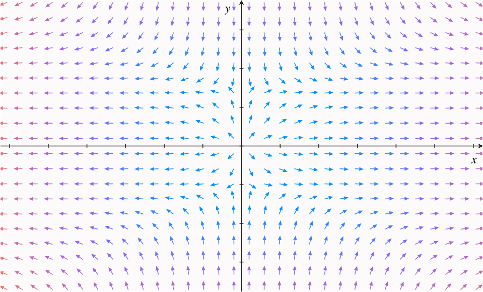
A sink on the other hand, is the opposite. Locations of sinks tell us where there are net negative charges in the field.

An example of a sink looks like the origin of this graph.

One thing to keep in mind

It's important to note that both of these vector fields might be snapshots of moments in time for their respective fields. You'll find gifs on the internet of vector fields in motion like this:

(This gif isn't mine and can be found here)

Think of the snapshots as depictions of the electric flux at a moment in time. Think of the gifs as the electric flux over a period of time. Electric flux doesn't have to remain constant.

Putting it all together

If we had a positive charge enclosed in a cube it would look something like this,

where the positive charge creates an electric field that "pushes" out from itself.

We are using a cube which acts as our closed, Gaussian surface. Remember, the charge doesn't have to actually be inside something solid and tangible; the cube doesn't have to exist in real life. Instead its shape and size are completely arbitrary. What matters is that the charge is completely enclosed within the surface.

Now we have this positive charge enclosed in the cube, which is exuding an electric field. Since it's positive, it will have a general outward flow of the electric field. If it were negative, the flow would be inward, towards the center of the cube.

Going back to the equation: the left side, $\oint \vec{E} \cdotp d\vec{A}$, describes the total amount of electric flux that is flowing out or into the surface and is normal to said surface. So if we took one of the electric lines, we'd try to get $d\vec{A}$ or the components of $E$ that are normal to the surface it crosses.

If we did that to all the lines, we'd get all of the normal components ($E_{n}$) of all the electric lines and thus all of the components of the electric flux that are directly leaving or entering the surface. The tangential components ($E_{t}$) don't matter since they don't contribute to what is leaving the surface.

To get all of the lines that are passing through the surface we would need to find the surface area of the enclosing shape and multiply by $\vec{E}$'s magnitude.

The right side of the equation involves finding the volume of the enclosing shape and using what we understand about how the charge might be distributed. Charge could be constantly distributed or based on a function, but the key factor is that the charge is distributed symettrically. Otherwise, using Gauss' Law would be painful.

But, bottom line, the left side of the equation is a surface area calculation with respect to the normal components of $\vec{E}$ and the right side is a volume calculation with respect to how the charges are distributed in the shape.

How do we apply this equation?

Now for a real example where we'll crunch some math. Let's say we have a distribution of charges within a sphere centered at the origin that follows $\rho(r) = \rho_{0}/r^2$ and we want to find the charge enclosed in a sphere of radius $r$.

Rho is used to represent the volume charge density which will help us calculate $Q_{enc}$. The function $\rho(r)$ is the charge density with respect to the radius $r$ where $\rho_{0}$ is the charge at the origin of the sphere. So as we go further and further away from the origin the charge density decreases because $r$ is inversely proportional.

We're going to use spherical coordinates ($r$, $\varTheta$, $\varPhi$) since we have a sphere. But now we have all these variables — $\rho$, $Q_{enc}$, $r$ — and we need figure out how they relate within Gauss Law.

$$\oint \vec{E} \cdotp d\vec{A} = Q_{enc}/\varepsilon_{0}$$

can be rewritten as

$$\varepsilon_{0} \oint \vec{E} \cdotp r^2 \sin \varTheta \enspace d\varPhi \enspace d\varTheta \enspace\hat{r} = Q_{enc}$$

because any vector normal to the the surface of the sphere is the $\hat{r}$ unit vector, which also corresponds to the component of $\vec{E}$ that we care about.

Since $E_{n}$ lines up with $\hat{r}$, this big jumble of letters — $r^2\sin\varTheta \enspace d\varPhi \enspace d\varTheta \hat{r}$ — won't matter.

We want all of the components of $\vec{E}$ that are normal to the sphere (all the $E_n$ as illustrated in the previous section). $\vec{E}$'s magnitude doesn't rely on $\varPhi$ or $\varTheta$; the angle of $\vec{E}$ doesn't change how strong or weak $\vec{E}$ is. The only thing that affects $\vec{E}$ is $r$. Therefore, since $\vec{E}$ is a function of $r$, we'll represent it like this: $\vec{E}_{n}(r)$.

(Pretend this is a sphere with lines shooting out of it)

This means we need to get the surface area of the sphere, which is $4\pi r^2$, and multiply it by $E_{n}(r)$:

$$4\pi r^2 \varepsilon_{0} \vec{E}_{n}(r) = Q_{enc}$$

Now for the right side of the equation. We want to get $Q_{enc}$ which is the charge inside of the sphere, a volume. Since we know the distribution of charge we can integrate over the sphere using our spherical coordinates:

$$4\pi r^2 \varepsilon_{0} \vec{E}_{n}(r) = \int_0^\pi \int_0^2\pi \int_0^r \rho_{0}/r^2 dr \, r \sin\varTheta \enspace d\varPhi \enspace r \enspace d\varTheta$$

Now we can solve.

$$\begin{align} 4\pi r^2 \varepsilon_{0} \vec{E}_{n}(r) &= \int_0^\pi \int_0^2\pi \int_0^r \rho_{0}/r^2 dr \, r \sin\varTheta \enspace d\varPhi \enspace r \enspace d\varTheta \\ &= \rho_{0} \int_0^\pi \int_0^2\pi \int_0^r \, dr \, \sin\varTheta \, d\varPhi \, d\varTheta \\ &= \rho_{0} \int_0^\pi \int_0^2\pi \lbrack r\rbrack^r_0 \, \sin\varTheta \, d\varPhi \, d\varTheta \\ &= r \rho_{0} \int_0^\pi \int_0^2\pi \sin\varTheta \, d\varPhi \, d\varTheta \\ &= r \rho_{0} \int_0^\pi \lbrack \varPhi \rbrack^2\pi_0 \, \sin\varTheta \, d\varTheta \\ &= 2\pi r \rho_{0} \lbrack -\cos\varTheta \rbrack^\pi_0 \\ &= 4\pi r \rho_{0} \end{align}$$

Simplification time:

$$\begin{aligned} 4\pi r^2 \varepsilon_{0} \vec{E}_{n}(r) &= 4\pi \, r \rho_{0} &\tt Remove \enspace 4\pi \nonumber \\ r^2 \varepsilon_{0} \vec{E}_{n}(r) &= r \rho_{0} &\tt Cancel \enspace out \enspace r \nonumber \\ \vec{E}_{n}(r) &= \rho_{0} / \varepsilon_{0} r \nonumber \end{aligned}$$

Since $\rho_{0}$ and $\varepsilon_0$ are constants, $\vec{E}_{n}(r)$ is inversely proportional to $r$. This makes sense since the further we go away from the origin and the center of the sphere the less charge there will be and, therefore, the less electric flux.

Why is it important?

In a nutshell, Gauss Law tells us:

• If there is no charge within an enclosed surface, there will be no electric flux out of that surface
• If there is a positive charge within an enclosed surface, then there will be a positive, outward flux leaving the surface
• If there is a negative charge within an enclosed surface, then there will be a negative, inward flux entering the surface

Engineers and scientists can use this law to determine the electric field for any symmetrical distribution of charges, so the contrived example where we counted charge from above would be difficult to calculate. Rather, examples that have cylindrical, spherical, or planar charge distributions such as capacitors or copper wires would be more appropriate applications of this equation.

Sources

• General overview of Gauss' Law
• A more mathy overview of Gauss' Law
• Khan Academy, whom I love
• This Youtube video